Steady flow system and first law of thermodynamics

Introduction

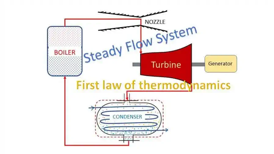
Flow processes occur in open system (control volume). Open system allows both mass and energy to cross the system boundary. We have already understood the applications of first law of thermodynamics to non-flow systems. Today we will discuss the applications of first law of thermodynamics to steady flow syatem. In a steady flow process a fluid flow steadily through a control volume. At any point of the flow, fluid properties remain constant during the process. There are many engineering equipments which function as steady flow system.

Flow energy

We have discussed that any moving mass may have kinetic energy (K.E.), potential energy (P.E.) and internal energy (I.E.). A flowing mass also have another form of energy called the flow energy (pv). This energy of flow moves the working substance across the boundary of open system is also known as flow work or displacement energy.

Assumption in the analysis of steady flow process

The following assumptions need to be made for analysis of steady flow energy system.

The mass flow is constant.
The state of the fluid at any point is constant with time.
The fluid composition is uniform.
Rate of heat and work transfer are constant.
Only potential energy (P.E), kinetic energy (K.E.), internal energy (I.E), and flow energy (pv) are considered for analysis.

Energy Equation for steady flow process

Let us consider the following steady flow system as shown in the figure.

The working substance of specific volume v_s1 enters the control volume at section 1-1 with a velocity of v₁ and at a pressure of p₁. The internal energy (I.E.) at section 1-1 is u₁ and the height of section is z₁ from the datum. Let the fluid leaves the control volume at section 2-2 with respective quantities v_s2, v₂, p₂, u₂ and z₂. As per the law of conservation of energy (first law of thermodynamics),

Total energy at section 1-1 = total energy at section 2-2

$Or,\ \ \ e_1=e_2$

$\left(PE\right)_1+\left(KE\right)_1+\left(IE\right)_1+\left(Flow\ Energy\right)_1+\left(Heat\ supplied\right)=\left(PE\right)_2+\left(KE\right)_2+\left(IE\right)_2+\left(Flow\ Energy\right)_2+\left(Work\ done\ \ by\ the\ system\ \right)$

$Or,\ \ z_1g+\frac{v_1^2}{2g}+u_1+p_1v_{s1}+q_{1-2}=z_2g+\frac{v_2^2}{2g}+u_2+p_2v_{s2}+w_{1-2}\rightarrow\left(i\right)$

By definition,

$Enthalpy,\ \ \ h=u+pv_s$

Therefore,

$z_1g+\frac{v_1^2}{2g}+\left(u_1+p_1v_{s1}\right)+q_{1-2}=z_2g+\frac{v_2^2}{2g}+\left(u_2+p_2v_{s2}\right)+w_{1-2}$

$Or,\ \ z_1g+\frac{v_1^2}{2g}+h_1+q_{1-2}=z_2g+\frac{v_2^2}{2g}+h_2+w_{1-2}\rightarrow\left(ii\right)$

Equation (ii) is called the steady flow energy equation which can also be written as:

$q_{1-2}-w_{1-2}=\left(z_2-z_1\right)g+\left(\frac{\left(v_2\right)^2-\left(v_1\right)^2}{2g}\right)+\left(h_2-h_1\right)$

$q_{1-2}-w_{1-2}=\left(pe_2-pe_1\right)+\left(ke_2-ke_1\right)+\left(h_2-h_1\right)$

In differential form the equation can be written as:

$\delta q\ -\delta\ w\ =d\left(pe\right)+d\left(ke\right)+dh$

In this system, heat is supplied (q_1-2 is positive) and work comes out of the system (w_1-2 is positive).

For a non-flow process,

$d\left(pe\right)=0,d\left(ke\right)=0,\ and\ d\left(pv_s\right)=0$

Therefore,

$\delta q\ -\delta\ w\ =du\ \ \ \left[since,\ dh=du+d\left(pv_s\right)=du\right]$

Work done in a steady flow system

In one of our previous blogs, we have discussed that work done in a non-flow process is,

$W_{1-2}=\int_{1}^{2}pdv$

The steady flow energy equation is,

$\delta q\ -\delta\ w\ =d\left(pe\right)+d\left(ke\right)+dh$

If change in potential and kinetic energy is zero,

$\delta q\ -\delta\ w\ =dh\rightarrow\left(i\right)$

From first law of thermodynamic for closed system is,

$\delta q\ =\ du\ +\ pdv\rightarrow\left(ii\right)$

We have already defined enthalpy as

$h\ =\ u\ +\ pv$

Differentiating we get,

$dh=du+pdv+vdp$

$dh=\left(du+pdv\right)+vdp$

$dh=\delta q+vdp\rightarrow\left(iii\right)\ \ \ \left(since,\delta q=du+pdv\right)$

Now equation (i) can be written as,

$\delta q\ -\ \delta w\ =\ \delta q\ +\ vdp$

$Or,\ \delta w\ =\ -\ vdp$

Integrating from state 1 to state 2 (see figure below),

$W_{1-2}=-\int_{1}^{2}vdp\rightarrow\left(iv\right)$

The non-flow and steady flow work and area under the curves are shown in the figure in a p-v diagram.

Work done in a Steady flow system during different processes

The applications of first law of thermodynamic to steady flow system involves study of different types of processes like isochoric, isobaric, isothermal etc. We will discuss them in brief.

Constant volume process (Isochoric)

$W_{1-2}=-\int_{1}^{2}vdp=-v\left(p_2-p_1\right)=v\left(p_1-p_2\right)$

Constant pressure process (Isobaric)

$W_{1-2}=-\int_{1}^{2}vdp=0\ \ \ since,dp=0$

Constant temperature process (Isothermal)

Workd done in a steady flow process,

$W_{1-2}=-\int_{1}^{2}vdp\rightarrow\left(i\right)$

For an isothermal process,

$pv=p_1v_1=p_2v_2=\ldots.constant$

$Or,\ v=\frac{p_1v_1}{p}$

Putting the value of v in equation (i)

$W_{1-2}=-\int_{1}^{2}vdp=-\int_{1}^{2}{\frac{p_1v_1}{p}dp}$

$W_{1-2}=-\int_{1}^{2}{\frac{1}{p}dp}$

$W_{1-2}=-p_1v_1.\left[{log}_e{p}\right]_1^2$

$W_{1-2}=-p_1v_1\left[{log}_e{p_2}-{log}_e{p_1}\right]$

$W_{1-2}=p_1v_1\left[\log_e{p_1}-\log_e{p_2}\right]$

$W_{1-2}=p_1v_1\log_e{\frac{p_1}{p_2}}$

$W_{1-2}=2.3\ p_1v_1\log{\frac{p_1}{p_2}}\rightarrow\left(ii\right)$

$Since,\ \frac{p_1}{p_2}=\frac{v_2}{v_1}$

$W_{1-2}=2.3\ p_1v_1log{\frac{v_2}{v_1}}\rightarrow\left(iii\right)$

Adiabatic process

We have,

$W_{1-2}=-\int_{1}^{2}vdp\rightarrow\left(i\right)$

The adiabatic law is,

$pv^\gamma=p_1v_1^\gamma=p_2v_2^\gamma=constant$

$Therefore,\ v=v_1p_1^{\frac{1}{\gamma}}.\frac{1}{p^\frac{1}{\gamma}}$

Putting the value of v in equation (i)

$W_{1-2}=-v_1p_1^{\frac{1}{\gamma}}.\int_{1}^{2}p^{\left(-\frac{1}{\gamma}\right)}dp$

After simplification we get,

$W_{1-2}=\frac{\gamma}{\gamma-1}\left[p_1v_1-p_2v_2\right]$

Polytropic process

The polytropic law is,

$pv^n=p_1v_1^n=p_2v_2^n=constant\ (n\ is\ polytropic\ index)$

The work done in a steady flow process for a polytropic process is,

$W_{1-2}=\frac{n}{n-1}\left[p_1v_1-p_2v_2\right]$

Engineering application of Steady flow energy equation

Now we will apply steady flow energy equation in different engineering devices used for various purposes.

Steam/Gas turbine: steady flow system

The steam turbine or gas turbine is a device to develop mechanical power output from heat energy. High pressure, high temperature steam/gas is allowed to expand in a turbine and a part of the energy is converted into work. The steam/gas leaves the turbine at lower pressure and low temperature. The figure explains the flow of working fluid and work output.

Applying steady flow energy equation at section 1 and 2,

$z_1g+\frac{v_1^2}{2g}+h_1+q_{1-2}=z_2g+\frac{v_2^2}{2g}+h_2+w_{1-2}$

In a turbine there is no heat transfer (q_1-2 = 0). The change in potential and kinetic energy are negligible (z₁ = z₂ and v₁ = v₂). Therefore,

$h_1=h_2+w_{1-2}$

$Or,\ \ w_{1-2}=h_1-h_2$

Rotary compressor: steady flow system

In a rotary compressor, air or gas is compressed and supply the same at high pressure. Figure shows the compressor with motor work input W_1-2. For such system, change in potential energy is generally zero.

Applying steady flow energy equation at section 1 and 2,

$z_1g+\frac{v_1^2}{2g}+h_1+q_{1-2}=z_2g+\frac{v_2^2}{2g}+h_2+w_{1-2}$

z₁ = z₂, if heat is lost from the system the q_1-2 is negative and also w_1-2 is negative (work done on the system)

$\frac{v_1^2}{2g}+h_1-q_{1-2}=\frac{v_2^2}{2g}+h_2-w_{1-2}$

If the compressor is insulated (q_1-2 =0) and change in kinetic energy is neglected (v₁ = v₂),

$h_1=h_2-w_{1-2}$

$Or,\ \ w_{1-2}=h_2-h_1$

Steam Boiler: steady flow system

Steam Boiler is an example of steady flow system. It is a closed vessel where water is heated by burning fuel to produce steam. Steam is used to run the steam turbine. The system of boiler is shown in the figure.

Applying steady flow energy equation at section 1 and 2,

$z_1g+\frac{v_1^2}{2g}+h_1+q_{1-2}=z_2g+\frac{v_2^2}{2g}+h_2+w_{1-2}$

For a boiler, z₁ = z₂ and v₁ = v₂. No work is done by a boiler (w_1-2 = 0) and heat is added to the system. Therefore,

$h_1+q_{1-2}=h_2$

$q_{1-2}=h_2-h_1$

Condenser: steady flow system

A steam condenser is used in a steam power plant. It converts the exhaust steam of the turbine to water by a process called condensation. Condenser is opposite of the process of boiler. Heat is extracted from the system and thus steam is converted to water (condensate). The system of condenser is shown in the figure.

Applying steady flow energy equation at section 1 and 2,

$z_1g+\frac{v_1^2}{2g}+h_1+q_{1-2}=z_2g+\frac{v_2^2}{2g}+h_2+w_{1-2}$

For a condenser, z₁ = z₂ and v₁ = v₂. No work transfer in a condenser (w_1-2 = 0) and heat is rejected by the system negative). Therefore,

$h_1-q_{1-2}=h_2$

$q_{1-2}=h_1-h_2$

Steam Nozzle: steady flow system

A steam nozzle is a passage of varying cross section to increase the kinetic energy of the fluid while the enthalpy as well as pressure drops. The part of the energy of steam is thus converted to kinetic energy to get a high velocity jet of steam. The system of convergent divergent nozzle is shown in the figure.

Applying steady flow energy equation at section 1 and 2,

$z_1g+\frac{v_1^2}{2g}+h_1+q_{1-2}=z_2g+\frac{v_2^2}{2g}+h_2+w_{1-2}$

In a steam nozzle, the is no heat and work transfer. z₁ = z_2.Therefore, Applying steady flow energy equation at section 1 and 2

$\frac{v_1^2}{2g}+h_1=\frac{v_2^2}{2g}+h_2$

$Or,\ \ v_2^2=v_1^2+2\left(h_1-h_2\right)$

$Or,\ \ v_2=\sqrt{v_1^2+2\left(h_1-h_2\right)}$

If exit velocity is vey large (v₂) than the inlet velocity (v₁), then v₁ can be neglected.

$v_2=\sqrt{2\left(h_1-h_2\right)}$

$Or,\ \ v_2=2∆h$

Steady flow system and first law of thermodynamics

Introduction

Flow energy

Assumption in the analysis of steady flow process

Energy Equation for steady flow process

Work done in a steady flow system

Work done in a Steady flow system during different processes

Constant volume process (Isochoric)

Constant pressure process (Isobaric)

Constant temperature process (Isothermal)

Adiabatic process

Polytropic process

Engineering application of Steady flow energy equation

Steam/Gas turbine: steady flow system

Rotary compressor: steady flow system

Steam Boiler: steady flow system

Condenser: steady flow system

Steam Nozzle: steady flow system

Thermodynamic System, definition, types and examples

Power Developed by Reciprocating IC Engine

APPLICATION OF FIRST LAW TO NON-FLOW PROCESS

Learn @ Home

System Interaction: Heat, Work and Energy

Gas Law and Gas Equation

Leave a Reply Cancel reply

More Links

Introduction

Flow energy

Assumption in the analysis of steady flow process

Energy Equation for steady flow process

Work done in a steady flow system

Work done in a Steady flow system during different processes

Constant volume process (Isochoric)

Constant pressure process (Isobaric)

Constant temperature process (Isothermal)

Adiabatic process

Polytropic process

Engineering application of Steady flow energy equation

Steam/Gas turbine: steady flow system

Rotary compressor: steady flow system

Steam Boiler: steady flow system

Condenser: steady flow system

Steam Nozzle: steady flow system

Similar Posts

Leave a Reply Cancel reply

More Links